Knowledge Base
Table of contents
Introduction
This knowledgeable base sets information about artificial intelligence, chemometrics and research data management together and combines this summary with small hands-on-tutorials. This compendium is only meant as a rough description and as starting point for work with the respective topics. In that sense the knowledge base is not meant to describe the topics extensively and the cited work is most often related to our work and therefore biased. Nevertheless, we hope the compendium is helpful and we added resources we found helpful.
Artificial Intelligence (AI)
According to R.E. Bellman (1978) artificial intelligence is the "[automation of] activities that we associate with human thinking, activities such as decision-making, problem solving, learning." With this broad definition the scientific fields of artificial intelligence features Greek ancient roots. Nevertheless, the first working AI programs were developed in the 1950’s and from this time also the term artificial intelligence (AI) originates. An important aspect of AI is machine learning (ML) and the first ML methods were developed in the field of statistics around 1900.
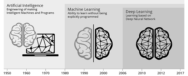
But what is "Machine learning (ML)"? ML is the science, which researches, develops and uses algorithms, statistical/mathematical methods that allow computer systems to improve their performance on a specific task. Machine learning methods either explicitly or implicitly construct a statistical/mathematical model of the data based on a sample dataset called "training data". Based on the underlying statistical/mathematical model ML methods can perform predictions or make decisions without being explicitly programmed to do so. This is the un-formal version of the famous and often quoted definition of ML by Tom M. Mitchell, 1997. ML techniques are utilized in a wide range of application ranging from spam detection in email accounts to computer vision and data analysis of spectroscopic data. Deep learning is a special type of machine learning methods, which were developed since 2006 and are often applied since 2010. These methods are composed of multiple layers of nonlinear processing units forming a high parameterized version of ML, which features a high degree of non-linearity. The difference between classical machine learning and deep learning is described in the respective sections.
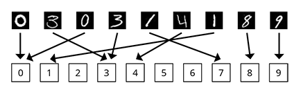
Like stated above machine learning is defined by Tom M. Mitchell (1997) as "a computer program is said to learn from experience E with respect to some class of tasks T and performance measure P, if its performance at tasks in T, as measured by P, improves with experience E". In order to make this clearer, we like to link it to the most prominent machine learning task. This often tested machine learning task is the following: A computer program should classify hand written digits (MNIST database of handwritten digits). In that respect the input of the model are images of size 28x28 pixels and the output of the model is one of the digits 0, 1, ... , 8, 9. This task (T) is visualized above and it gives an instructive example of the working of ML methods for image recognition. The experience E are the know ground truth for the trainings data, e.g. the known connection between the training images and the numbers. The performance measure is some error rate between the ML prediction and the ground truth. We utilize these ML and Deep Learning methods similarly to elucidate the difference between bio-medical conditions of samples, which are characterized by spectral or image measurements.
Machine Learning (ML)
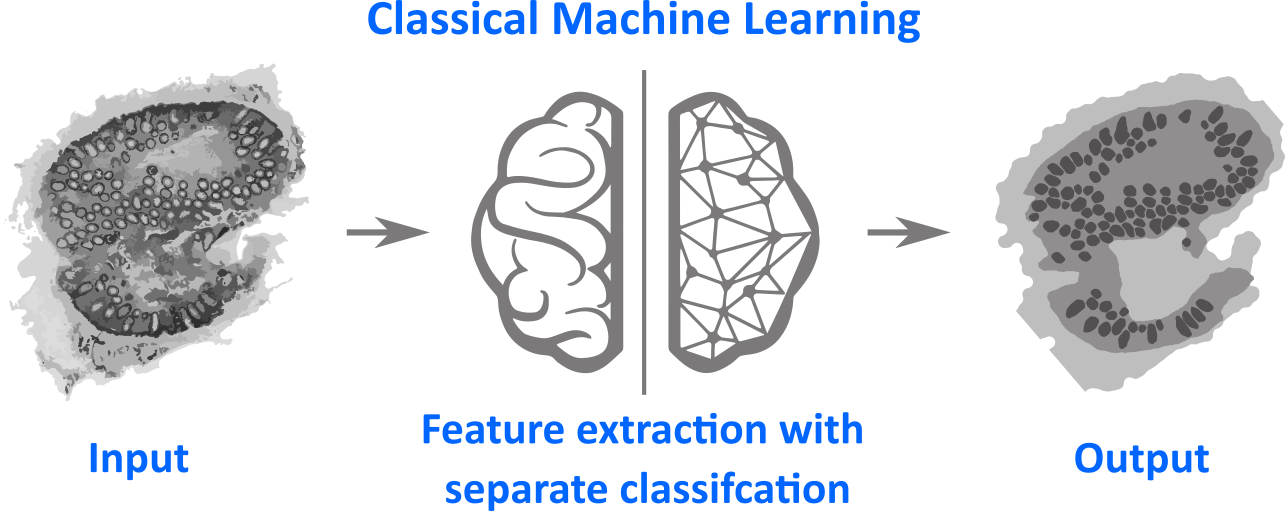
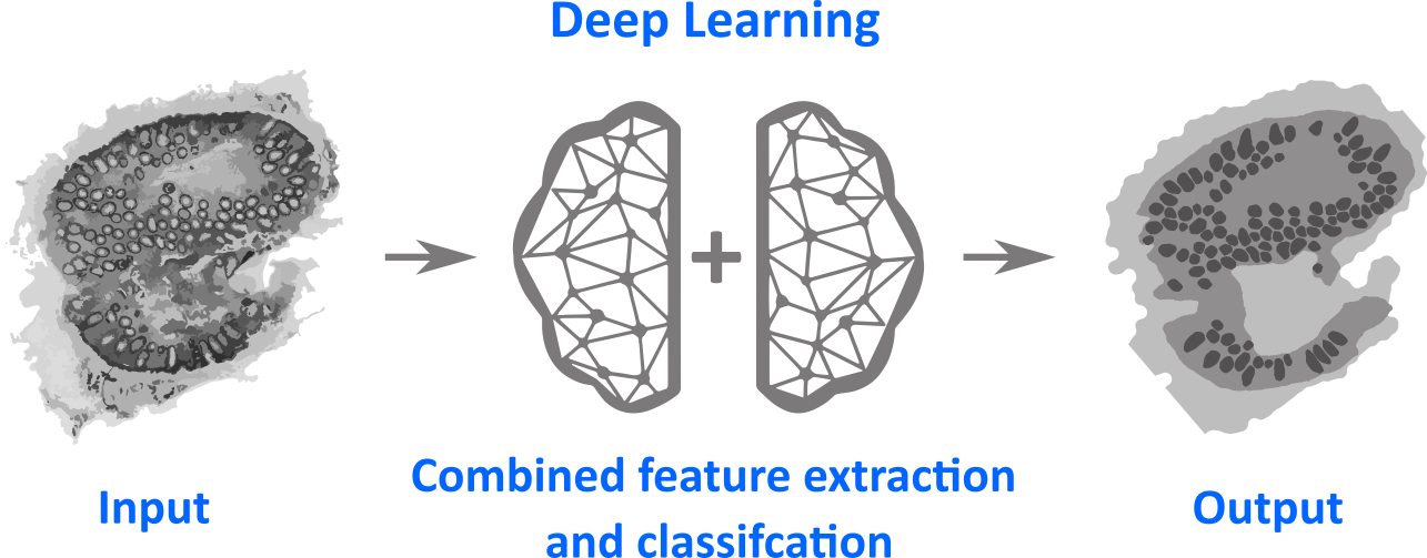
In classical machine learning (CML) the link between the images and higher information about this data, e.g class labels, is carried out in a two-step procedure. In the first step image features are extracted. The concrete types of image features are designed by a researcher using his/her knowledge and intuition about the samples and data at hand. Therefore human intervention is needed for this feature extraction. After the features are extracted the (multivariate) dataset is analyzed using easy classification models, like linear discriminant analysis (LDA).
This procedure is sketched in the figure above. A multimodal image is used as input image and the desired output is an image with three gray levels: one indicating background pixel and the other both gray levels represent different tissue classes. Therefore the machine learning task is to perform the translation between both images and is called semantic segmentation. After the image features ware extracted the so called training data set is used to train the classification model, where a number of images together with their true tissue segmentation is known.
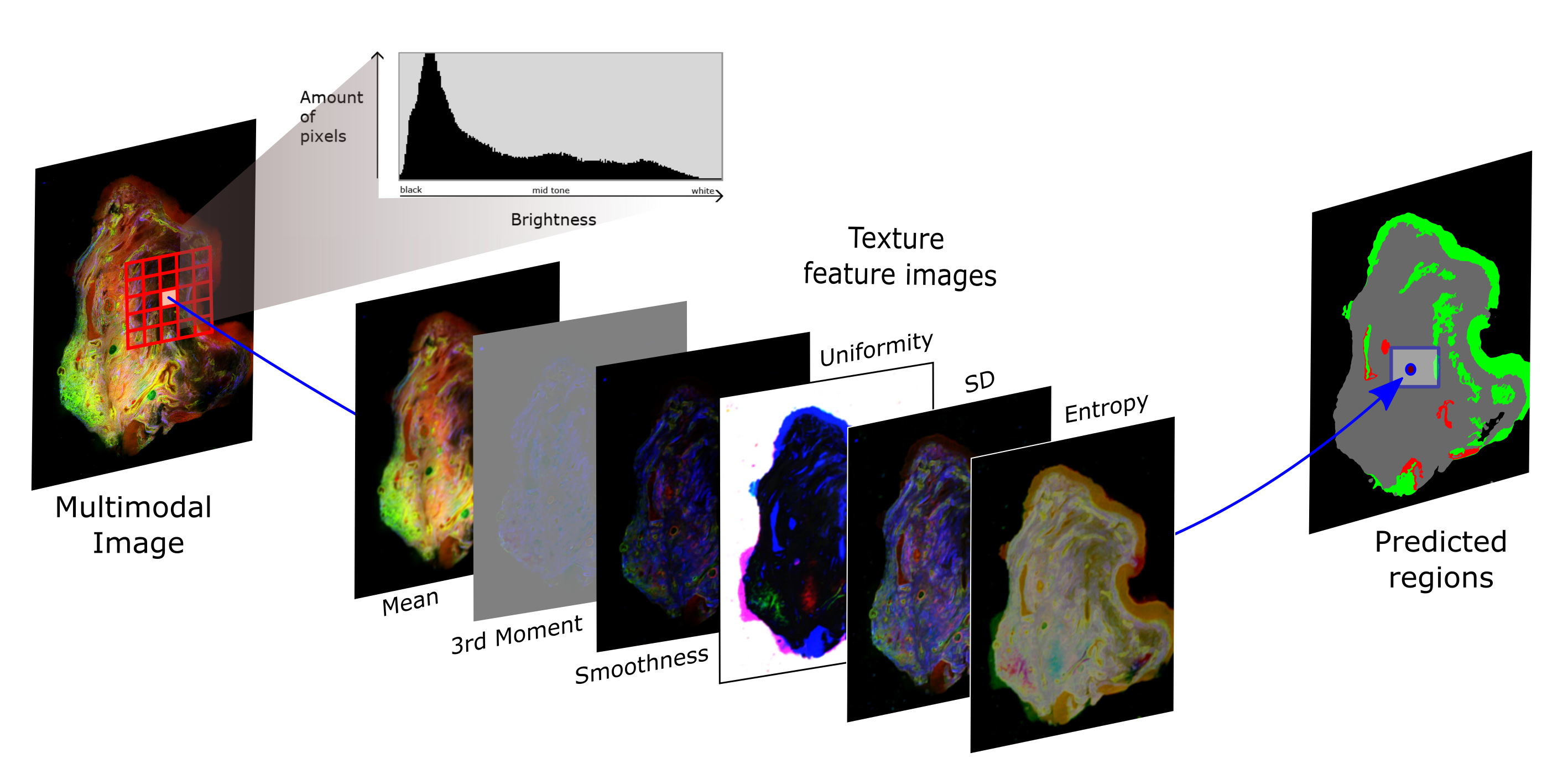
In the figure above a classical machine learning framework is visualized for the study of Heuke et al. (2016). The multimodal images (left side) are utilized to calculate statistical moments of the histogram in a local mode, which characterize the texture. In a region around a central pixel the histogram of the image values is calculated. Based on that first order statistical moments or derivate of them, like mean, standard deviation and entropy, are calculated and this is performed on every pixel of the image as central pixel. In that way feature images (mid part of the figure) are generated which are subsequently utilized to predict, which tissue regions are present at the central pixel. The results are false color images like shown on the right of the above figure, where green represents healthy epithelium, while red indicates cancerous areas.
Publications of the group
- Guo S, Pfeifenbring S, Meyer T, Ernst G, von Eggeling F, Maio V, Massi D, Cicchi R, Pavone F S, Popp J, Bocklitz T (2018) Multimodal Image Analysis in Tissue Diagnostics for Skin Melanoma. Journal of Chemometrics 32:e2963. DOI: 10.1002/cem.2963
- Moawad A A, Silge A, Bocklitz T, Fischer K, Rösch P, Roesler U, Elschner M C, Popp J, Neubauer H (2019) A Machine Learning-Based Raman Spectroscopic Assay for the Identification of Burkholderia mallei and Related Species. Molecules 24:4516. DOI: 10.3390/molecules24244516
- Yarbakht M, Pradhan P, Köse-Vogel N, Bae H, Stengel S, Meyer T, Schmitt M, Stallmach A, Popp J, Bocklitz T W, Bruns T (2019) Nonlinear Multimodal Imaging Characteristics of Early Septic Liver Injury in a Mouse Model of Peritonitis. Analytical Chemistry 91:11116–11121. DOI: 10.1021/acs.analchem.9b01746
- Guo S, Silge A, Bae H, Tolstik T, Meyer T, Matziolis G, Schmitt M, Popp J, Bocklitz T (2021) FLIM data analysis based on Laguerre polynomial decomposition and machine-learning. Journal of Biomedical Optics 26:1-13. DOI: 10.1117/1.JBO.26.2.022909
Useful resources
Deep Learning (DL)
Deep Learning is a special version of machine learning, which is inspired by the working of the human brain in processing of visual data or other kinds of input. Deep learning for semantic segmentation is visualized in the figure above. The main property of deep learning is that the feature extraction is done by the method implicitly in combination with the construction of a classification model. This is the main advantage, because no human is needed to construct a suitable feature extraction. The drawback is that these models can’t be interpreted and the model has a lot of parameters (typically 1Mio parameters). Nevertheless, these models feature a unique potential to solve a large class of machine learning tasks, especially if a large amount of data is existing.
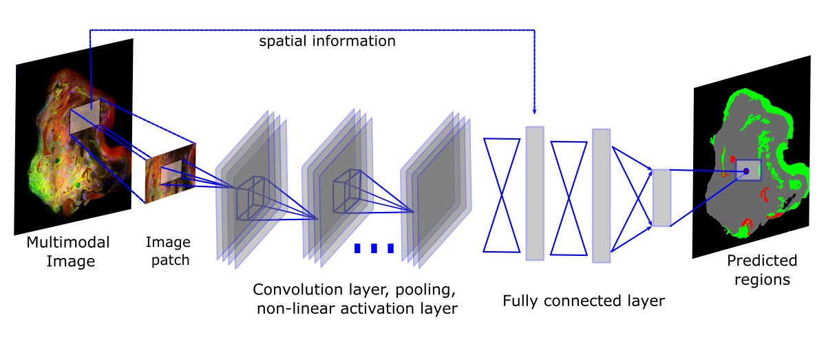
In the figure above a special kind of deep learning method, a convolutional neuronal network is visualized (CN24 architecture pre-trained using the ILSVRC2012 dataset). It adapts the processing of visual input by the human brain, by performing a large number of subsequent convolutional operations. Therefore, the main part of these networks consists of convolutional filters applied subsequently to generate feature images, which are subsequently converted into class prediction. Again a local prediction of tissue types based on multimodal images is generated using this network, which can be seen on right of the figure. The deep learning technique can be seen as non-linear translation tool from the multimodal images (left side) into the false color images characterizing the tissue types (right side).
Publications of the group
- Pradhan P, Meyer T, Vieth M, Stallmach A, Waldner M, Schmitt M, Popp J, Bocklitz T (2019) Semantic segmentation of Non-Linear Multimodal images for disease grading of Inflammatory Bowel Disease – A SegNet-based application. In: Proceedings of the 8th International Conference on Pattern Recognition Applications and Methods - Volume 1: ICPRAM. SciTePress, pp 396–405. DOI: 10.5220/0007314003960405
- Ali N, Quansah E, Köhler K, Meyer T, Schmitt M, Popp J, Niendorf A, Bocklitz T (2019) Automatic Label-free Detection of Breast Cancer Using Nonlinear Multimodal Imaging and the Convolutional Neural Network ResNet50. Translational Biophotonics 1:e201900003. DOI: 10.1002/tbio.201900003
- Guo S, Mayerhöfer T, Pahlow S, Hübner U, Popp J, Bocklitz T (2020) Deep learning for ’artefact’ removal in infrared spectroscopy. Analyst 145:5213–5220. DOI: 10.1039/D0AN00917B
- Ali N, Kirchhoff J, Onoja P I, Tannert A, Neugebauer U, Popp J, Bocklitz T (2020) Predictive Modeling of Antibiotic Susceptibility in E. Coli Strains Using the U-Net Network and One-Class Classification. IEEE Access 8:167711–167720. DOI: 10.1109/ACCESS.2020.3022829
- Houhou R, Barman P, Schmitt M, Meyer T, Popp J, Bocklitz T (2020) Deep learning as phase retrieval tool for CARS spectra. Optics Express 28:21002–21024. DOI: 10.1364/OE.390413
- Kirchberger-Tolstik T, Pradhan P, Vieth M, Grunert P, Popp J, Bocklitz T W, Stallmach A (2020) Towards an interpretable classifier for characterization of endoscopic Mayo scores in ulcerative colitis using Raman Spectroscopy. Analytical Chemistry online:1–10. DOI: 10.1021/acs.analchem.0c02163
- Pradhan P, Köhler K, Guo S, Rosin O, Popp J, Niendorf A, Bocklitz T W (2021) Data Fusion of Histological and Immunohistochemical Image Data for Breast Cancer Diagnostics using Transfer Learning. In: Proceedings of the 10th International Conference on Pattern Recognition Applications and Methods - Volume 1: ICPRAM,. SciTePress, pp 495–506 DOI: 10.5220/0010225504950506
Useful resources
Chemometrics
The field of science that is focused on data-driven extraction of information from chemical systems is called chemometrics. Chemometrics is inherently interdisciplinary as methods of data science and multivariate statistics are applied in chemistry, biology, or medicine. Besides classical statistical and machine learning tasks, chemometrics also includes spectral data cleansing, calibration, and standardization. These steps are often very specific to the analyzed data type and require understanding of the underlying measurement techniques and the respective corrupting effects. Another important part of spectroscopic data analysis is the establishment of robust evaluation of supervised models. Such evaluation requires both proper design of experiments and careful implementation of a model validation pipeline. Therefore, experimental design and evaluation procedures are also considered to be a part of chemometrics.
Publications of the group
- Bocklitz, T., Schmitt, M., Popp, J., 2014. Image Processing—Chemometric Approaches to Analyze Optical Molecular Images, in: Ex-Vivo and In-Vivo Optical Molecular Pathology. John Wiley & Sons, Ltd, pp. 215–248. DOI: 10.1002/9783527681921.ch7
- Houhou, R., Bocklitz, T., n.d. Trends in artificial intelligence, machine learning, and chemometrics applied to chemical data. Anal. Sci. Adv. n/a. DOI: 10.1002/ansa.202000162
- Ryabchykov, O., Guo, S., Bocklitz, T., 2019. Analyzing Raman spectroscopic data. Phys. Sci. Rev. 4, 20170043. DOI: 10.1515/psr-2017-0043
Useful resources
- Brereton, R.G., Jansen, J., Lopes, J., Marini, F., Pomerantsev, A., Rodionova, O., Roger, J.M., Walczak, B., Tauler, R., 2017. Chemometrics in analytical chemistry—part I: history, experimental design and data analysis tools. Anal. Bioanal. Chem. 409, 5891–5899. DOI: 10.1007/s00216-017-0517-1
Pretreatment
Prior to analyzing spectral data of a sample, the contribution of corrupting effects originating from external effects and the measurement device must be suppressed. The steps of data pretreatment are highly dependent on the used measurement technique and the setup. The spectroscopic methods that employ CCD/CMOS sensors and require long acquisition times, such as Raman spectroscopy, may need cosmic ray spikes correction. Most of spectral techniques require calibration or correction of the device response function. The required calibration methods may differ largely because they depend not only on the employed measurement technique, but also on the experimental design.
Publications of the group
- Ryabchykov, O., Bocklitz, T., Ramoji, A., Neugebauer, U., Foerster, M., Kroegel, C., Bauer, M., Kiehntopf, M., Popp, J., 2016. Automatization of spike correction in Raman spectra of biological samples. Chemom. Intell. Lab. Syst. 155, 1–6. DOI: 10.1016/j.chemolab.2016.03.024
- Bocklitz, T.W., Dörfer, T., Heinke, R., Schmitt, M., Popp, J., 2015. Spectrometer calibration protocol for Raman spectra recorded with different excitation wavelengths. Spectrochim. Acta. A. Mol. Biomol. Spectrosc. 149, 544–549. DOI: 10.1016/j.saa.2015.04.079
Useful resources
- Gibb, S., Strimmer, K., 2012. MALDIquant: a versatile R package for the analysis of mass spectrometry data. Bioinformatics 28, 2270–2271. DOI: 10.1093/bioinformatics/bts447
Preprocessing
Common steps in spectral data preprocessing are baseline correction and normalization of the spectra. Although the underlying effect leading to the spectral background are different in different spectroscopic and spectrometric techniques, the same methods are often employed for the baseline estimation. Thus, statistics-sensitive non-linear Iterative peak-clipping (SNIP) algorithm was introduced for X-ray spectra preprocessing but is also widely used for removing chemical noise background in mass spectrometry and correcting of the fluorescence background in Raman spectroscopy. Besides baseline correction, spectra often need normalization to further standardize the spectra. There is a variety of normalization methods available, but the choice of the method depends both on the employed technique and the intendent application.
Alternative preprocessing approach common for vibrational spectroscopy is a model-based extended multiplicative signal correction (EMSC), which standardizes the background and the signal intensity according to a given reference. This approach is especially robust for homogeneous data sets but may not be optimal if the spectra within the data set are too diverse.
Publications of the group
- Guo, S., Bocklitz, T., Popp, J., 2016. Optimization of Raman-spectrum baseline correction in biological application. Analyst 141, 2396–2404. DOI: doi.org/10.1039/C6AN00041J
Useful resources
- Ryan, C.G., Clayton, E., Griffin, W.L., Sie, S.H., Cousens, D.R., 1988. SNIP, a statistics-sensitive background treatment for the quantitative analysis of PIXE spectra in geoscience applications. Nucl. Instrum. Methods Phys. Res. Sect. B Beam Interact. Mater. At. 34, 396–402. DOI: 10.1016/0168-583X(88)90063-8
- Skogholt, J., Liland, K.H., Indahl, U.G., 2019. Preprocessing of spectral data in the extended multiplicative signal correction framework using multiple reference spectra. J. Raman Spectrosc. 50, 407–417. DOI: 10.1002/jrs.5520
Data modeling
Even after proper preprocessing, analysis of the spectral data might be challenging due to the high dimensionality of data. In order to extract useful information from the spectra, multivariate statistics and machine learning are commonly used. As in other machine learning fields, popular modeling methods in chemometrics need to be robust, but the distinctive feature of chemometric methods is the model interpretability. Understanding of the spectral features that contribute to the model prediction helps to additionally ensure the model robustness and stability. In some tasks, especially in research, interpretable models can provide deeper understanding of the underlying processes. Besides typical machine learning tasks, such as classification, regression, clustering, and segmentation, chemometrics also specializes in spectral unmixing, multiway methods, segmentation of hyperspectral images, and analysis of process dynamics.
Publications of the group
- Guo, S., Rösch, P., Popp, J., Bocklitz, T., 2020. Modified PCA and PLS: Towards a better classification in Raman spectroscopy–based biological applications. J. Chemom. 34, e3202. DOI: 10.1002/cem.3202
- Hniopek, J., Schmitt, M., Popp, J., Bocklitz, T., 2020. PC 2D-COS: A Principal Component Base Approach to Two-Dimensional Correlation Spectroscopy. Appl. Spectrosc. 74, 460–472. DOI: 10.1177/0003702819891194
Useful resources
- Brereton, R.G., 2015. Pattern recognition in chemometrics. Chemom. Intell. Lab. Syst. 149, 90–96. DOI: 10.1016/j.chemolab.2015.06.012
- Dagher, I., 2010. Incremental PCA-LDA algorithm, in: 2010 IEEE International Conference on Computational Intelligence for Measurement Systems and Applications. Presented at the 2010 IEEE International Conference on Computational Intelligence for Measurement Systems and Applications, pp. 97–101. DOI: 10.1109/CIMSA.2010.5611752
- Indahl, U.G., Liland, K.H., Næs, T., 2009. Canonical partial least squares—a unified PLS approach to classification and regression problems. J. Chemom. 23, 495–504. DOI: 10.1002/cem.1243
Model transfer
A typical challenge for the supervised predictive models constructed on the spectral data is application of the model to the data measured on a different device or after replacing components of the device. Even slight variations between the device components may introduce device-specific effects, which may make it impossible to directly use the model constructed on the data from one measurement device to a different device. To overcome this issue, model transfer methods can be applied. Usually, the model transfer methods require a few reference spectra from each device in order to tune the model. Besides the transfer of the predictive model itself, the transfer may be done in the model-based preprocessing (such as EMSC) by using the same reference and introduction of interferent spectrum.
Publications of the group
- Guo, S., Heinke, R., Stöckel, S., Rösch, P., Popp, J., Bocklitz, T., 2018a. Model transfer for Raman-spectroscopy-based bacterial classification. J. Raman Spectrosc. 49, 627–637. DOI: 10.1002/jrs.5343
- Guo, S., Kohler, A., Zimmermann, B., Heinke, R., Stöckel, S., Rösch, P., Popp, J., Bocklitz, T., 2018b. Extended Multiplicative Signal Correction Based Model Transfer for Raman Spectroscopy in Biological Applications. Anal. Chem. 90, 9787–9795. DOI: 10.1021/acs.analchem.8b01536
Useful resources
Fan, W., Liang, Y., Yuan, D., Wang, J., 2008. Calibration model transfer for near-infrared spectra based on canonical correlation analysis. Anal. Chim. Acta 623, 22–29. DOI: 10.1016/j.aca.2008.05.072
Workman, J.J., 2018. A Review of Calibration Transfer Practices and Instrument Differences in Spectroscopy. Appl. Spectrosc. 72, 340–365. DOI: 10.1177%2F0003702817736064
Evaluation methods
In order to validate supervised predictive models a few different approaches can be used. The most robust and the simplest approach from the data processing pipeline design is the split of the data set into 3 independent subsets: training, validation, and test sets. Then the model can be constructed on the training data set, optimized according to the predictions on the validation data set, and finally, get tested on the test data. Unfortunately, the approach with 3 independent data sets also requires a significant amount of data, which might not be easily accomplished in practice. With limited number of samples, cross-validation approaches can be employed for model optimization, when at each step of the cross-validation loop the data is resampled into large training subset and a smaller validation subset. In order to keep the cross-validation robust, it is important to keep the subsets independent. Furthermore, to emulate training-validation-test approach, a 2-level cross validation approach should be implemented, when the inner loop is used for model optimization and the outer loop is only used for the model testing.
Publications of the group
- Ali, N., Girnus, S., Rösch, P., Popp, J., Bocklitz, T., 2018. Sample-Size Planning for Multivariate Data: A Raman-Spectroscopy-Based Example. Anal. Chem. 90, 12485–12492. DOI: 10.1021/acs.analchem.8b02167
- Guo, S., Bocklitz, T., Neugebauer, U., Popp, J., 2017. Common mistakes in cross-validating classification models. Anal. Methods 9, 4410–4417. DOI: 10.1039/C7AY01363A
Useful resources
- Arlot, S., Celisse, A., 2010. A survey of cross-validation procedures for model selection. Stat. Surv. 4, 40–79. DOI: 10.1214/09-SS054
- Balluff, B., Hopf, C., Porta Siegel, T., Grabsch, H.I., Heeren, R.M.A., 2021. Batch Effects in MALDI Mass Spectrometry Imaging. J. Am. Soc. Mass Spectrom. 32, 628–635. DOI: 10.1021/jasms.0c00393
2D correlation analysis
Soon ...
Research data management (RDM)
Research data management (RDM) is the process of transformation, selection and storage of research data with the aim of keeping the data accessible, reusable and verifiable in the long term and independent of the data producer. These requirements are further specified and the FAIR principle was introduced, which stands for findable accessible, interoperable and reusable. RDM can be understood as process support the research data lifecycle to fulfill the FAIR requirements. The national research data (National Forschungsdateninfrastruktur Initiative, NFDI) is the national process to develop a RDM for all scientific disciplines in Germany.
In detail the FAIR principles state the following.
- Data should be findable: That means data should be findable by humans and machines, which requires machine-readable and writable metadata enabling somebody to find records.
- Data should be accessible: A long-term archiving with standard communication protocols that can be used by humans and machines is needed to allow a (long-term) access of the data.
- Data should be interoperable: Choose a format that makes the data or parts of it automatically exchangeable, interpretable and combinable with other data sets.
- Data should be reusable: Only by a good description of data and metadata a reuse is possible. The conditions of use need to be specified in a way that is understandable for people and machines, which allows proper data citation.
Publications of the group
- Steinbeck et al. NFDI4Chem - Towards a National Research Data Infrastructure for Chemistry in Germany Research Ideas and Outcomes, Pensoft Publishers, 2020, 6, e55852, DOI: 10.3897/rio.6.e55852
Useful resources
- Homepage of the National Research Data Infrastructure (NFDI)
- Homepage of the NFDI4Chem: Chemistry Consortium in the NFDI
- German information on RDM: Forschungsdaten.info
- Overview on Open Scince: Open-Science-Training-Handbook
- Overview on Open Scince: Fosteropenscience.eu
- Karl W. Broman & Kara H. Woo (2018) Data Organization in Spreadsheets, The American Statistician, 72:1, 2-10, DOI: 10.1080/00031305.2017.1375989
- Wilkinson et al. The FAIR Guiding Principles for scientific data management and stewardship Scientific data, 2016, 3, DOI: 10.1038/sdata.2016.18
Research data and metadata
Research data are (digital) data that are generated during scientific activity (e.g. through measurements, surveys, …). Research data form the basis of scientific work and document scientific findings. This fact results in a discipline- and project-specific understanding of research data with different requirements for the preparation, processing and management of the data: the so-called research data management (RDM). Sometimes a distinction is made between primary research data or primary data and metadata, although the latter are often not considered research data in the strict sense, depending on the discipline.
Primary research data are collected raw data that have neither been edited nor commented on or provided with metadata, but which form the basis for the scientific study of an object. The distinction between research data and primary research data can sometimes only be made theoretically, because the latter are never published without minimal metadata or otherwise remain incomprehensible. Thus, digitized material is never published by its owners, e.g. scientific libraries and collections, without background information such as provenance and the like.
Metadata is independent data that contains structured information about other data or resources and their characteristics. They are stored independently of or together with the data they describe in more detail. A precise definition of metadata is difficult because, on the one hand, the term is used in different contexts and, on the other hand, the distinction between data and metadata varies depending on the point of view. Usually a distinction is made between content metadata and technical or administrative metadata. While the latter have a clear metadata status, domain-oriented metadata can sometimes also be understood as research data. To increase the effectiveness of metadata, a standardization of the description is absolutely necessary. A metadata standard allows metadata from different sources to be linked and edited together.
Data life cycle
This is a sub paragraph, formatted in heading 3 style: Lorem ipsum dolor sit amet, consectetuer adipiscing elit. Aenean commodo ligula eget dolor. Aenean massa. Cum sociis natoque penatibus et magnis dis parturient montes, nascetur ridiculus mus. Donec quam felis, ultricies nec, pellentesque eu, pretium quis, sem. Nulla consequat massa quis enim. Donec pede justo, fringilla vel, aliquet nec, vulputate
Ontology
This is a sub paragraph, formatted in heading 3 style: Lorem ipsum dolor sit amet, consectetuer adipiscing elit. Aenean commodo ligula eget dolor. Aenean massa. Cum sociis natoque penatibus et magnis dis parturient montes, nascetur ridiculus mus. Donec quam felis, ultricies nec, pellentesque eu, pretium quis, sem. Nulla consequat massa quis enim. Donec pede justo, fringilla vel, aliquet nec, vulputate
Electronic Lab Notebook (ELN)
This is a sub paragraph, formatted in heading 3 style: Lorem ipsum dolor sit amet, consectetuer adipiscing elit. Aenean commodo ligula eget dolor. Aenean massa. Cum sociis natoque penatibus et magnis dis parturient montes, nascetur ridiculus mus. Donec quam felis, ultricies nec, pellentesque eu, pretium quis, sem. Nulla consequat massa quis enim. Donec pede justo, fringilla vel, aliquet nec, vulputate
Database
This is a sub paragraph, formatted in heading 3 style: Lorem ipsum dolor sit amet, consectetuer adipiscing elit. Aenean commodo ligula eget dolor. Aenean massa. Cum sociis natoque penatibus et magnis dis parturient montes, nascetur ridiculus mus. Donec quam felis, ultricies nec, pellentesque eu, pretium quis, sem. Nulla consequat massa quis enim. Donec pede justo, fringilla vel, aliquet nec, vulputate
Repository
This is a sub paragraph, formatted in heading 3 style: Lorem ipsum dolor sit amet, consectetuer adipiscing elit. Aenean commodo ligula eget dolor. Aenean massa. Cum sociis natoque penatibus et magnis dis parturient montes, nascetur ridiculus mus. Donec quam felis, ultricies nec, pellentesque eu, pretium quis, sem. Nulla consequat massa quis enim. Donec pede justo, fringilla vel, aliquet nec, vulputate
Smart Lab
This is a sub paragraph, formatted in heading 3 style: Lorem ipsum dolor sit amet, consectetuer adipiscing elit. Aenean commodo ligula eget dolor. Aenean massa. Cum sociis natoque penatibus et magnis dis parturient montes, nascetur ridiculus mus. Donec quam felis, ultricies nec, pellentesque eu, pretium quis, sem. Nulla consequat massa quis enim. Donec pede justo, fringilla vel, aliquet nec, vulputate
Tutorials
In this section, hands-on-tips, FAQs and information about data handling workflows are set together, which are rather specific to the photonic data science group. You might find some information and tips useful, but this section isn't meant in a general way.
OMERO: Upload Data
OMERO is client-server software for managing, visualizing and analyzing (microscopic) images and associated metadata. OMERO allows you to upload and archive your images in converted format within the server repository. There are two main interfaces for OMERO: a desktop client (OMERO.insight) and a webpage (OMERO.web). Importing data into OMERO will be mainly done using OMERO.insight desktop client. You can work with your images using a desktop app (Windows, Mac or Linux) or programming languages as well as ImageJ.
OMERO: Upload Metadata
If you want to use your OMERO imported images for scientific purposes, it is crucial to access the image metadata. Every image exhibit a large amount of metadata, which define experimental and data acquisition conditions, analytic results, annotations and other information relevant to the image data. Metadata is essential for interpretation of the image data. For example, how the image was recorded, information about pixel type, data dimensions, and many other information. As images are uploaded to OMERO, the associated metadata contained in the image file will automatically imported (we call this experimental metadata). However, beside the experimental metadata, additional metadata can be provided in a separate txt file or xlsx file along with your images. This is often needed for sample related metadata, which is normally not automatically recorded during an experiment. This kind of metadata do not import automatically while importing images into OMERO. In this case you need to start from a local CSV file and end up with a OMERO.table using server-side populate metadata script in OMERO.web.
ElabFTW: Generate metadata tables
This is a sub paragraph, formatted in heading 3 style: Lorem ipsum dolor sit amet, consectetuer adipiscing elit. Aenean commodo ligula eget dolor. Aenean massa. Cum sociis natoque penatibus et magnis dis parturient montes, nascetur ridiculus mus. Donec quam felis, ultricies nec, pellentesque eu, pretium quis, sem. Nulla consequat massa quis enim. Donec pede justo, fringilla vel, aliquet nec, vulputate
Handling metadata using spreadsheets
Spreadsheets are widely used software tools for data entry, storage, analysis, and visualization. These programs can be used to organize data and metadata to reduce errors and ease later analyses. It is important to keep the primary (data and metadata) files pristine and data-only. Calculations and visualizations should be done in separate files. The primary concern of these data and metadata files is to protect the integrity of the data and/or metadata, and to ease later analysis. The following tips are taken from Broman et al. and they make life easier:
- Be Consistent
- Choose Good Names for Things
- Write Dates as YYYY-MM-DD
- No Empty Cells: Put ‘NA’ or even a hyphen in the cells with missing data, to make it clear that the data are known to be missing rather than unintentionally left blank.
- Put Just One Thing in a Cell: Don’t have ‘plate-well’ such as ‘13-A01’ as column but ‘plate’ and ‘well’ separately.
- Make it a Rectangle
- Create a Data Dictionary: Explain you variables, units and names / terms used in the file
- No Calculations in the raw data / metadata files
- Do not use font color or highlighting as data / metadata
- Make backups
- Use data validation to avoid errors (within the spreadsheet program in use)
- Save the Data in Plain Text Files: The CSV format is not pretty to look at, but you can open the file in Excel or another spreadsheet program and view it in the standard way.
Useful resources
- Karl W. Broman & Kara H. Woo (2018) Data Organization in Spreadsheets, The American Statistician, 72:1, 2-10, DOI: 10.1080/00031305.2017.1375989